Lab 5: Linear PID Control + Linear Extrapolation

I placed the main ToF and PID behavior inside a Bluetooth command case instead of running it directly in loop(). This let me start a test from Python, collect data for a fixed number of iterations, and send the saved arrays back over Bluetooth for plotting.

In GET_ALL, the robot runs through the control loop, stores time, ToF distance, PID output, and error terms in arrays, then sends the saved data back after the run. I also made an END_PID command to stop the run early.

case GET_ALL:
{
  const unsigned long starttime = millis();
  Serial.println("Start Collecting Data");

  ToF_Sensor_1.startRanging();
  ToF_Sensor_2.startRanging();

  for (int i = 0; i < Acc_length; i++)
  {
    BLEDevice central = BLE.central();

    if (central) {
      if (central.connected()) {
        write_data();
        read_data();
      }
    }

    if (!PID_state) break;

    // sensor read + PID + array logging
  }

  PID_state = true;
  ToF_Sensor_1.stopRanging();
  ToF_Sensor_2.stopRanging();
  stop_motors();
  break;
}

case END_PID:
{
  PID_state = false;
  ToF_Sensor_1.stopRanging();
  ToF_Sensor_2.stopRanging();
  stop_motors();
  break;
}

The goal was to have the robot drive toward a wall and stop at a setpoint of 12 inches. The main challenge was balancing speed and stability so the robot moved quickly without overshooting into the wall.

I started with proportional control only and tested Kp = 0.1, 3, 3.5, and 4. At Kp = 0.1 the response was too weak. At Kp = 3 the robot moved toward the wall but felt slow. At Kp = 4 it became too aggressive and touched the wall.

I chose Kp = 3.5 as a good starting point. Later, after more tuning with integral and derivative action, I also tested a stronger final setup.

distance1_in = distance1 * 0.0393701f;
error1P = distance1_in - targetDistance1;

float control = kp * error1P + ki * error1I + kd * error1D;
duty1 = abs(control);

After tuning Kp, I added a deadband to reduce oscillation near the setpoint. Small motor commands were not always enough to overcome friction, so the robot could jitter close to the target.

In my code, the deadband was set to 0.75 inches. Inside that range, the robot stops; otherwise it drives forward or backward depending on the sign of the error.

float deadband = 0.75;

if (fabs(error1P) < deadband) {
    stop_motors();
    dutystate = 0;
}
else if (error1P > 0) {
    drive_forward(duty1);
    dutystate = 1;
}
else {
    drive_backward(duty1);
    dutystate = -1;
}

I then tested integral gain values of 0.02, 0.01, 0.005, and 0.002. These were harder to tune because even small changes caused noticeable differences in behavior. I also tested derivative control to reduce overshoot as the robot approached the wall.

A combined starting point I used was Kp = 3.5, Ki = 0.02, and Kd = 0.8. After more tuning, I ended up testing Kp = 5, Ki = 0.01, and Kd = 1.0.

error1I = error1I + error1P * PID_dt * (-1);

if (PID_dt > 0) {
    error1D = (error1P - error1Plast) / PID_dt;
} else {
    error1D = 0;
}

error1Plast = error1P;
if (error1I > 4000) error1I = 4000;
if (error1I < -4000) error1I = -4000;

The ToF sensor updates slower than the main control loop, so I did not want the controller to block and wait for a new reading every iteration. Instead, my code checks whether new ToF data is ready and only updates the saved distance when a fresh measurement is available.

My ToF Sensors take around 50-60 ms to update, while my main PID control loop runs around 158.8 loops per second (about 6.3 ms per loop). This means the controller can run multiple iterations between ToF updates, which is why non-blocking logic is important.

I kept the extrapolation discussion here because that is the next step for improving performance between sensor updates, but the current code below shows the non-blocking ToF update logic I actually used.

// Linear extrapolation for ToF distance when no new sensor data is ready

if (ToF_Sensor_1.checkForDataReady()) {
  float distance1 = ToF_Sensor_1.getDistance();
  ToF_Sensor_1.clearInterrupt();

  distance1_in = distance1 * 0.0393701f;   // mm -> inches
  distance1_est = distance1_in;            // update latest estimate
}
else if (i > 1) {
  // Use the last two saved distance points to estimate current distance
  float x1 = Tof1_in[i - 2];
  float x2 = Tof1_in[i - 1];

  float t1 = time_list[i - 2] / 1000.0f;   // ms -> s
  float t2 = time_list[i - 1] / 1000.0f;   // ms -> s
  float t_now = (float)(millis() - starttime) / 1000.0f;

  if ((t2 - t1) > 0.0001f) {
      float slope = (x2 - x1) / (t2 - t1);
      distance1_est = x2 + slope * (t_now - t2);
  }
  else {
      distance1_est = x2;
  }

  distance1_in = distance1_est;
}

For the 5000-level version of the lab, I also considered integrator wind-up. This happens when the integral term keeps building while the motors are saturated or the robot cannot respond well, which can cause extra overshoot later.

In my code, I handled this by clamping the accumulated integral error to a fixed range.

error1I = error1I + error1P * PID_dt * (-1);

if (error1I > 4000) error1I = 4000;
if (error1I < -4000) error1I = -4000;

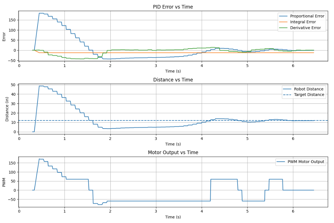
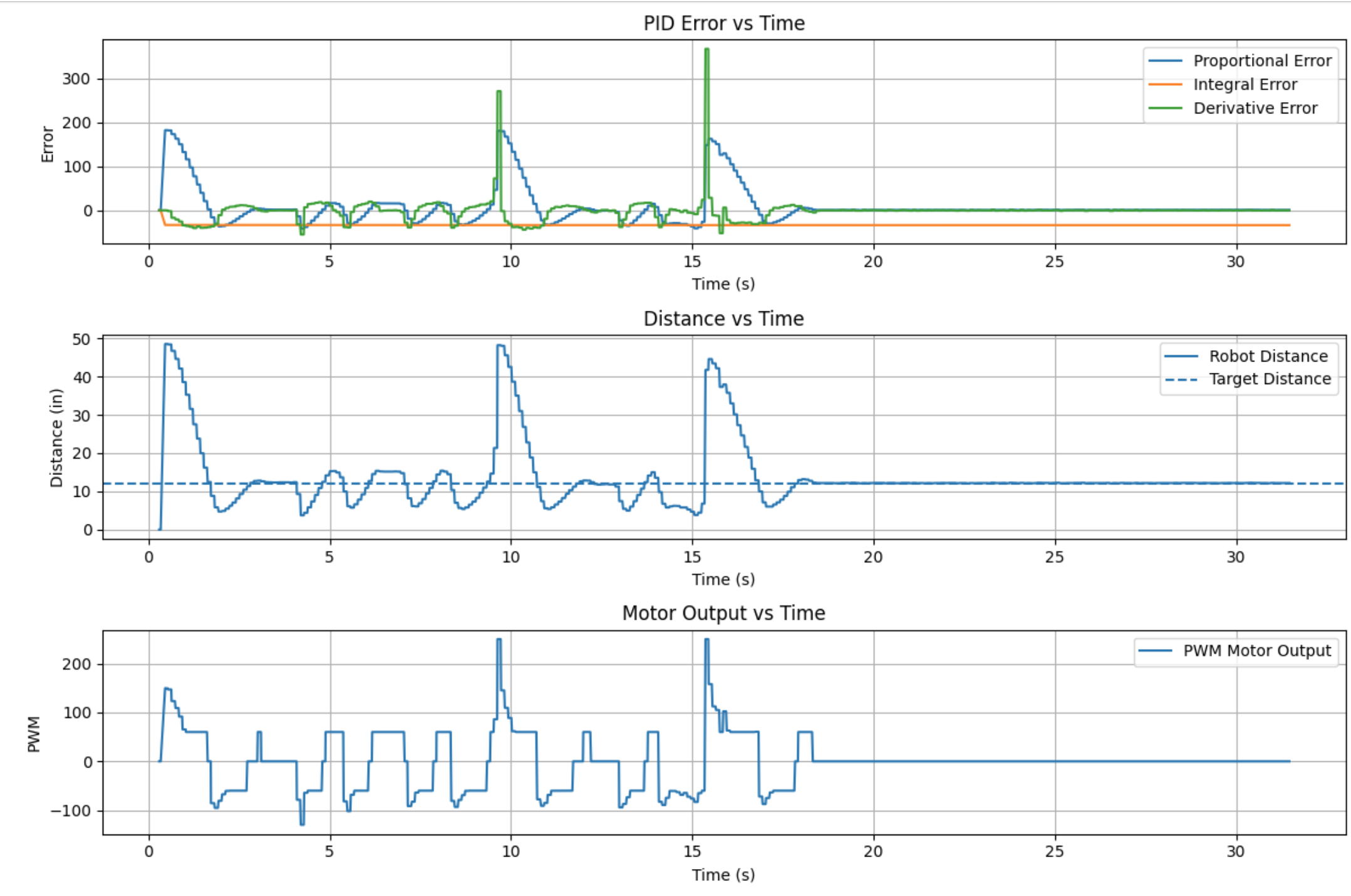
The plots below should show how the robot approached the wall, how close it got to the 12 inch setpoint, and how the motor commands changed during the run. I also included placeholders for repeated test videos.

Kp = 5.0, Ki = 0.01, Kd = 1.0

With Random Input

Overall, this lab showed how controller tuning, sensor timing, and practical motor limits affect real robot behavior. My early proportional tuning showed that Kp = 3.5 was a good starting point, and later tuning with Kp = 5, Ki = 0.01, and Kd = 1.0 gave a stronger final response. Deadband logic improved behavior near the setpoint, and clamping the integral term helped prevent wind-up.