Lab 6: Orientation Control with IMU + PD
In this lab I used the IMU gyroscope and DMP yaw estimate to control the robot’s orientation.
1. Prelab: Bluetooth Debugging Setup
To send and receive data over Bluetooth while the controller was running, I set up a command structure
in the Arduino code named GET_PID_ORI_GAINS_AND_ORIENTATION. This let me send gain
values and target orientation data to the Arduino. I also added lines to
tx_estring_value.append so the robot could send logged values back to my computer for
post-processing.
The code below shows how I sent values to the Arduino and then sent values back to my computer.
Bluetooth Gain / Setpoint Command
case GET_PID_ORI_GAINS_AND_ORIENTATION:
{
  bool Received_input = robot_cmd.get_next_value(kp_ori)
                     && robot_cmd.get_next_value(ki_ori)
                     && robot_cmd.get_next_value(kd_ori)
                     && robot_cmd.get_next_value(targetOrientation1);
  if (!Received_input) return;

  tx_estring_value.clear();
  tx_estring_value.append("PID Ori Gains are Set, kp_ori = ");
  tx_estring_value.append(kp_ori);
  tx_estring_value.append(", ki_ori = ");
  tx_estring_value.append(ki_ori);
  tx_estring_value.append(", kd_ori = ");
  tx_estring_value.append(kd_ori);
  tx_estring_value.append(", Target Orientation = ");
  tx_estring_value.append(targetOrientation1);

  tx_characteristic_string.writeValue(tx_estring_value.c_str());
  break;
}
The next code block shows how I received values back on my computer and parsed them for plotting and analysis.
Python Call Example
def notif_handler(uuid, byte):
  s = ble.bytearray_to_string(byte)
  parts = s.split("|")

  PID_ori      = float(parts[14])
  Perror_ori   = float(parts[15])
  Ierror_ori   = float(parts[16])
  Derror_ori   = float(parts[17])
  PWM_ori      = float(parts[18])

  PID_ori_list.append(PID_ori)
  Perror_ori_list.append(Perror_ori)
  Ierror_ori_list.append(Ierror_ori)
  Derror_ori_list.append(Derror_ori)
  PWM_ori_list.append(PWM_ori)

PID_ori_list      = []
Perror_ori_list   = []
Ierror_ori_list   = []
Derror_ori_list   = []
PWM_ori_list      = []

ble.start_notify(ble.uuid['RX_STRING'], notif_handler)
ble.send_command(CMD.GET_ALL, "")
2. Orientation Control Goal
The goal of this lab was to have the robot rotate to a desired heading and stop there with a stable response. The main challenge was balancing speed and stability so the robot turned quickly enough without overshooting too much or oscillating around the setpoint.
3. IMU Input Signal and Orientation Estimate
To estimate the robot’s orientation, gyroscope data needs to be integrated over time. Digital integration sums angular velocity measurements over discrete time steps to estimate the rotation angle. A problem with this is that even small errors in angular velocity can build up over time and cause drift.
In my implementation, I used the IMU’s onboard Digital Motion Processor (DMP) and converted the quaternion output into yaw. This gave a cleaner heading estimate and helped reduce yaw drift compared to using a simple raw gyro integration by itself.
Yaw Estimate From DMP Quaternion Data
icm_20948_DMP_data_t data;
myICM.readDMPdataFromFIFO(&data);

if ((myICM.status == ICM_20948_Stat_Ok) ||
    (myICM.status == ICM_20948_Stat_FIFOMoreDataAvail)) {

  if ((data.header & DMP_header_bitmap_Quat6) > 0) {

    double q1 = ((double)data.Quat6.Data.Q1) / 1073741824.0;
    double q2 = ((double)data.Quat6.Data.Q2) / 1073741824.0;
    double q3 = ((double)data.Quat6.Data.Q3) / 1073741824.0;
    double q0 = sqrt(1.0 - ((q1 * q1) + (q2 * q2) + (q3 * q3)));

    double qw = q0;
    double qx = q2;
    double qy = q1;
    double qz = -q3;

    double t3 = +2.0 * (qw * qz + qx * qy);
    double t4 = +1.0 - 2.0 * (qy * qy + qz * qz);
    Gyro_yaw = (float)atan2(t3, t4) * 180.0 / PI + 3.8;
  }
}
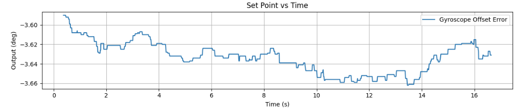
I also needed to calibrate the yaw value so it displayed a more accurate heading. I let the DMP run
while the robot stayed still and watched the yaw drift until it reached a steady-state value around
-3.6 to -3.9 degrees. Based on that, I added a calibration offset of +3.8 degrees.
Calibration at +3.8 Degrees
4. P and D Gain Tuning
For this lab, I tested proportional and derivative control. Proportional control determined how strongly the robot reacted to error, while derivative control helped reduce overshoot and made the turning response more damped. I did not use integral control because PD already did a good enough job.
PD Controller Logic From My Code
error1P_ori = Gyro_yaw - targetOrientation1;

unsigned long now = millis();
PID_dt_ori = (now - PID_time2_ori) / 1000.0;
PID_time2_ori = now;

if (PID_dt_ori > 0) {
  error1D_ori = (error1P_ori - error1Plast_ori) / PID_dt_ori;
} else {
  error1D_ori = 0;
}

error1Plast_ori = error1P_ori;

control_ori = (kp_ori * error1P_ori) + (kd_ori * error1D_ori);
duty2 = abs(control_ori);

if (duty2 < duty1Min_ori) duty2 = duty1Min_ori;
if (duty2 > duty1Max_ori) duty2 = duty1Max_ori;
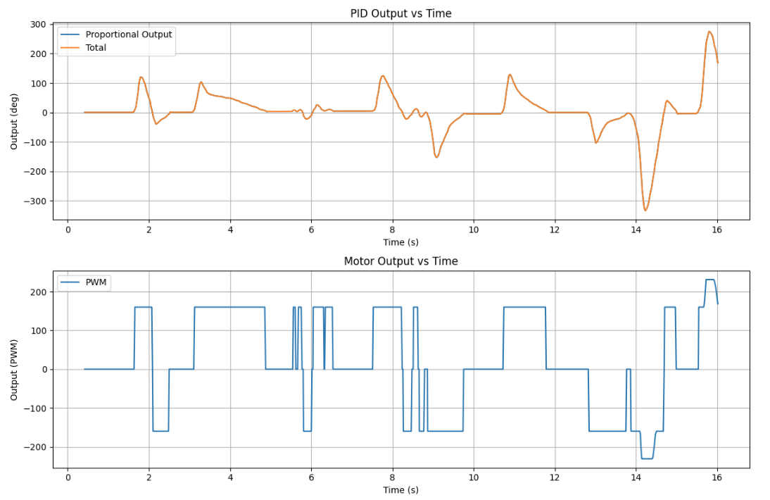
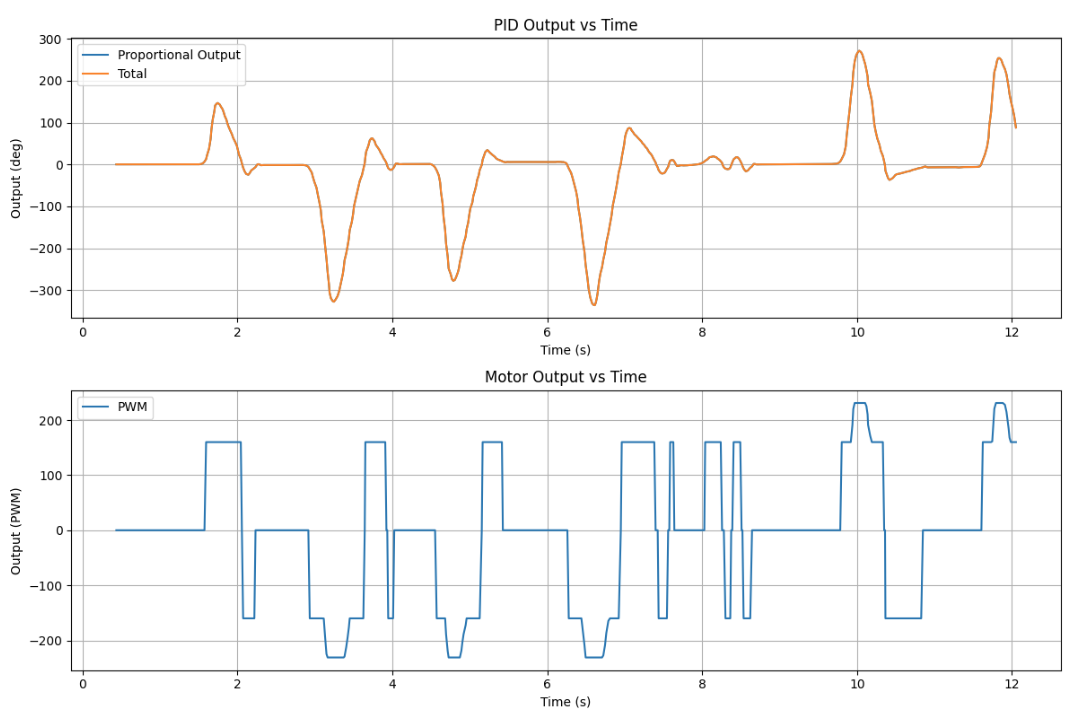
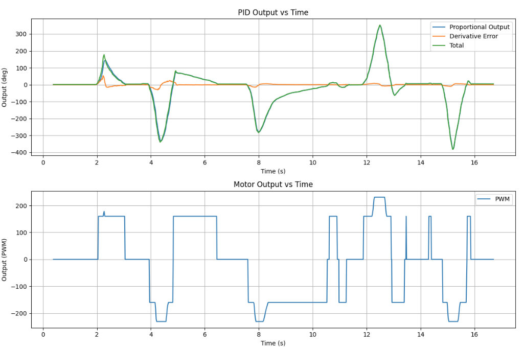
These plots show the first three tests I ran with different proportional gains:
Kp = 3.0, Kp = 3.75, and Kp = 4.5.
I ended up using Kp = 3.75 because it gave decent corrective angular velocity while
keeping the overshoot relatively low.
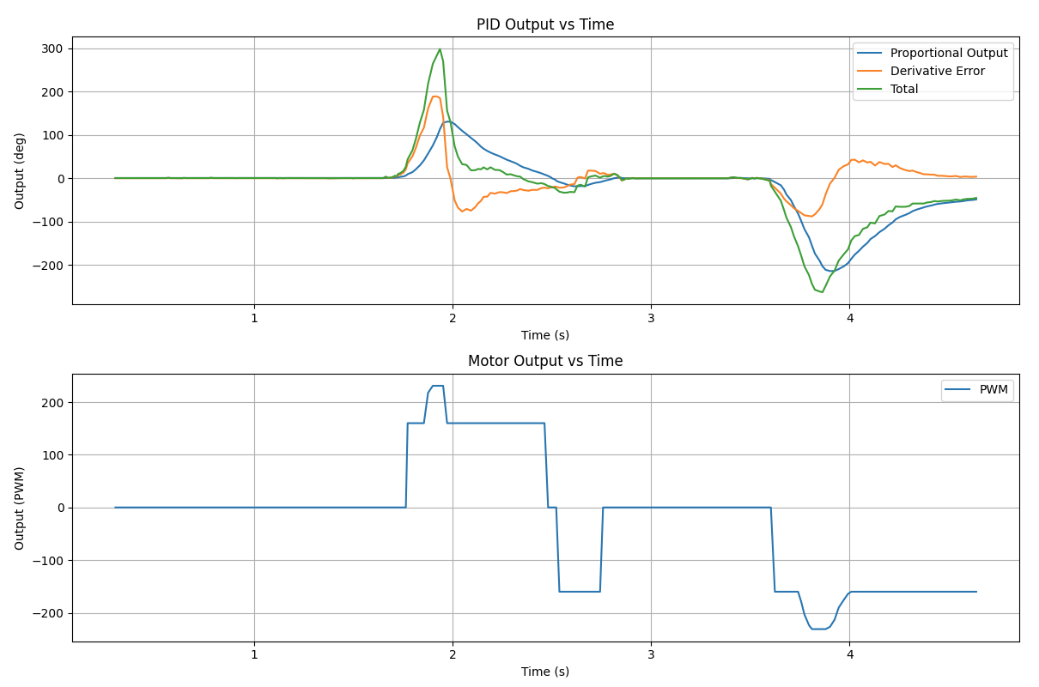
Test 1: Kp = 3.0
Test 2: Kp = 3.75
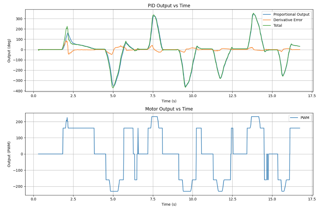
Test 3: Kp = 4.5
Test Video: Kp = 3.75
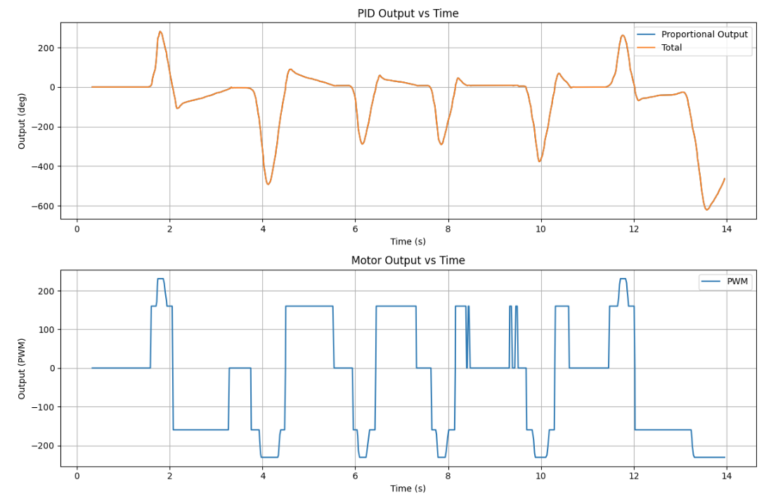
These next plots show the first three tests I ran with different derivative gains:
Kd = 20, Kd = 40, and Kd = 60.
I ended up using Kd = 40 because it damped the aggressive angular acceleration and
reduced overshoot compared to Kd = 20, while still keeping better corrective angular
velocity than Kd = 60, which was a bit too damped.
Test 1: Kd = 20
Test 2: Kd = 40
Test 3: Kd = 60
Test Video: Kd = 40
5. Deadband and Motor Command Logic
After tuning the turning gains, I added a deadband near the target heading so the robot would stop once it was close enough instead of constantly trying to correct tiny remaining errors. Without this, the robot could keep twitching back and forth near the setpoint.
In my code, the deadband for orientation was set to 2 degrees. If the robot was
inside that range, the motors stopped. Otherwise, the robot turned left or right depending on the sign
of the error.
Deadband Logic From My Code
float deadband_ori = 2.0;

if (fabs(error1P_ori) <= deadband_ori) {
  stop_motors();
  dutystate_ori = 0;
  ori_finish = 1;
}
else {
  ori_finish = 0;

  if (error1P_ori > 0) {
    turn_right(duty2);
    dutystate_ori = 1;
  }
  else {
    turn_left(duty2);
    dutystate_ori = -1;
  }
}
Turning Functions
void turn_right(float duty1motor) {
  float cali = 1.1;
  duty1motor = (int)abs(duty1motor);
  int duty2motor = (int)fabs(duty1motor * cali);

  analogWrite(PWM_0, duty1motor);
  analogWrite(PWM_1, 0);
  analogWrite(PWM_2, duty2motor);
  analogWrite(PWM_5, 0);
}

void turn_left(float duty1motor) {
  float cali = 1.1;
  duty1motor = (int)abs(duty1motor);
  int duty2motor = (int)fabs(duty1motor * cali);

  analogWrite(PWM_0, 0);
  analogWrite(PWM_1, duty1motor);
  analogWrite(PWM_2, 0);
  analogWrite(PWM_5, duty2motor);
}
6. Derivative Term and Sampling Time Discussion
The derivative term was useful for reducing overshoot, but it is also sensitive to noise. Since the heading estimate comes from IMU data, fast noise in the signal can make the derivative term jump around. In practice, derivative action works best when the signal is reasonably smooth.
Another thing that matters is the timestep. The derivative term depends on dt, so if the
sampling time is inconsistent, then the derivative estimate will also be inconsistent. That is why I
tracked time during the loop and used it directly in the controller calculations.
To find the sampling rate I took a loop of 1000 indexes and found the amount of time it took to run the loop.
The timestamp value I recieved was 16.64s. Meaning that this loop ran at around 60 loops per second.
Changing the setpoint while the robot is running can also create derivative kick, since the derivative term reacts strongly to rapid changes in error. For future improvements, filtering or derivative-on-measurement would help make the controller even smoother.
Timing in the Control Loop
const unsigned long starttime = millis();

for (int i = 0; i < Acc_length; i++)
{
  const uint32_t t_us = micros();

  // IMU read
  // BLE processing
  // controller update
  // array logging

  time_list[i] = (float)(millis() - starttime);
}
7. Wind-Up Protection
For the 5000-level part of the lab, wind-up protection is still important to discuss even though I did not use integral control in the final PD controller. Integrator wind-up happens when the integral term keeps growing while the motors are saturated or the robot cannot respond well, which can lead to larger overshoot later.
In my code, I included clamping logic for the integral term. If I had kept integral control in the final implementation, this would help prevent the accumulated error from becoming too large.
Wind-Up Clamp From My Code
error1I_ori += error1P_ori * PID_dt_ori;

if (error1I_ori > 4000) error1I_ori = 4000;
if (error1I_ori < -4000) error1I_ori = -4000;