Lab 7 | MAE 5190 Fast Robots

1. Objective

The goal of this lab was to use a Kalman Filter to supplement the slower Time of Flight sensor measurements with a model-based estimate of the robot’s state. This allows the robot to better estimate both position and velocity between ToF updates and improves the behavior from Lab 5.

2. Step Response Data Collection

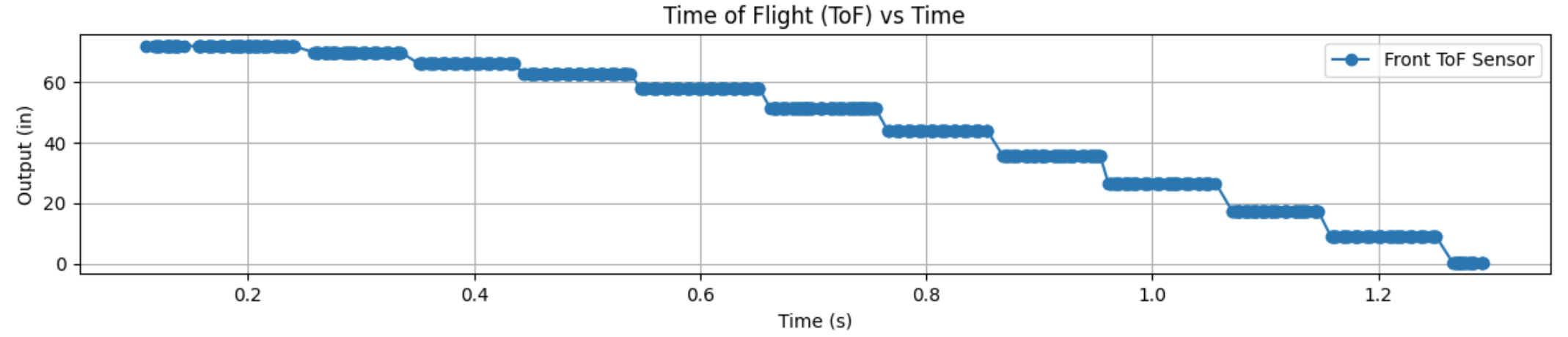
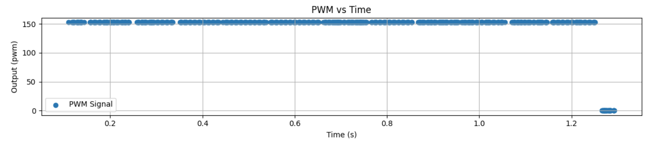
To estimate the system dynamics, I drove the robot toward the wall at a constant motor input of 152 PWM and logged the ToF output, motor input, and timing data. I used my Bluetooth debugging structure again so I could run the robot, save the values in arrays, and then send those values back to Jupyter for analysis.

This step response data was used to estimate the rise time and overall system behavior, which I later used to build the A and B matrices for the Kalman Filter.

Bluetooth Data Logging Structure

case GET_ALL:
{
  const unsigned long starttime = millis();
  Serial.println("Start Collecting Data");

  for (int i = 0; i < Acc_length; i++)
  {
    BLEDevice central = BLE.central();

    if (central) {
      if (central.connected()) {
        write_data();
        read_data();
      }
    }

    if (!PID_state) break;

    if (ToF_Sensor_1.checkForDataReady()) {
      int distance1 = ToF_Sensor_1.getDistance();
      ToF_Sensor_1.clearInterrupt();
      distance1_in = distance1 * 0.0393701f;

      time_list[i] = (float)(millis() - starttime);
      Tof_Sensor_1_list[i] = distance1_in;
      PWM_list[i] = duty1;
    }
  }
  break;
}

Data Collection Video

3. Velocity and Rise Time Estimation

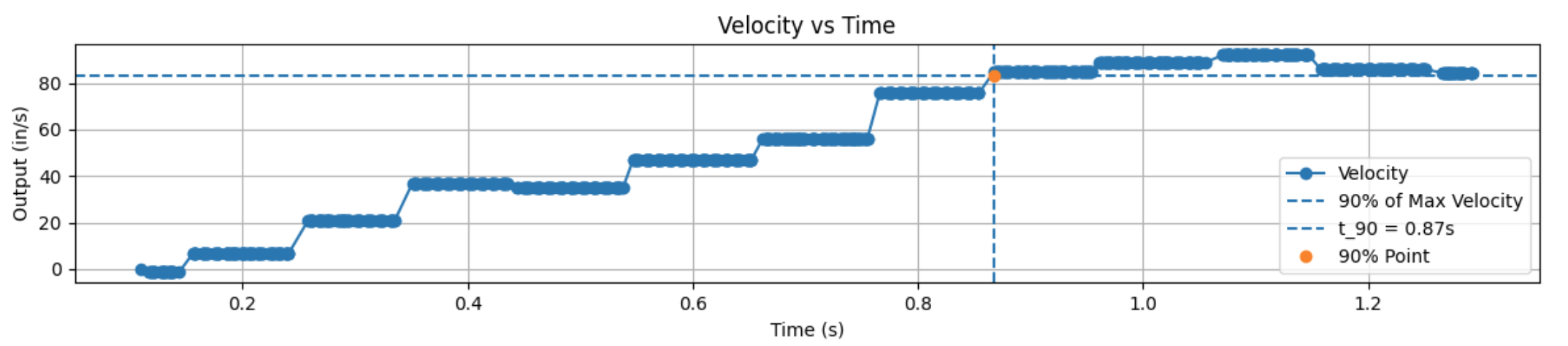
After collecting the ToF distance data, I computed the robot’s forward velocity in Python by taking the derivative of position with respect to time. This let me analyze the step response in terms of velocity instead of only position.

From the velocity response, I estimated the rise time and used the 90% value of the maximum speed to identify the response speed of the system. My measured rise time was about 0.868 s.

I also looked at the loop timing. I had 13 definitive datapoints in 1.229 s, which corresponds to about 10.6 loops per second. That means each loop took about 0.0945 s per iteration.

Python Logic for 90% Rise Time

max_vel = max(Forward_Velocity_list[:1100])
vel_90 = 0.9 * max_vel

axs[1].axhline(y=vel_90, linestyle='--', label='90% of Max Velocity')

for i, v in enumerate(Forward_Velocity_list[:1100]):
    if v >= vel_90:
        Time_90 = time_list[i]
        break

4. State Space Model Setup

Once I had the step response information, I used it to estimate the drag: 0.0066719 and momentum: 0.0022717 behavior of the robot and build the state space model. The states I used were distance from the wall and velocity.

System Model and Parameter Estimation

m * dv/dt = -d*v + u

Steady State:
0 = -d*v_ss + u
d = u / v_ss

Time Constant:
tau = t_90 / 2.3

Momentum Term:
m = d * tau

State Space Representation

State Vector:
x = [position, velocity]
A = [ 0      1
      0   -d/m ]
B = [ 0
      1/m ]
C = [ -1   0 ]

After estimating the model, I discretized the A and B matrices using the sample time. The C matrix was chosen so that the measured output corresponded to the ToF distance reading.

Discrete System Form

Ad = np.eye(n) + Delta_T * A
Bd = Delta_T * B
C = np.array([[-1, 0]])
x = np.array([[-TOF[0]], [0]])

I also had to choose covariance matrices for the process noise and sensor noise. These values control how much the filter trusts the model versus the measured sensor data.

Measurement Noise


Σ_z = [ σ₃² ]

σ₃² = (20 mm)²

Process Noise (Dependent on Sampling Time)


Σ_u = [ σ₁²   0
         0   σ₂² ]

Sampling Time


Δt ≈ 0.0945 s

Trust in Modeled Position & Velocity


σ₁ = σ₂ = √(10² · (1 / Δt))

σ₁ = σ₂ =√(100 / 0.0945)

σ₁ ≈ σ₂ ≈ 32.5 mm

Covariance Matrix Setup

sig_u = np.array([[sigma_1**2, 0],
                  [0, sigma_2**2]])

sig_z = np.array([[sigma_3**2]])

5. Kalman Filter in Python

Before putting the Kalman Filter on the robot, I first implemented it in Jupyter. This made it easier to check that the model and covariance values made sense before moving everything over to the Artemis.

The Kalman Filter works in two main steps: prediction and correction. The model predicts the next state, and then the measured ToF value is used to correct that prediction.

Kalman Filter Function

def kf(mu, sigma, u, y):

    mu_p = A.dot(mu) + B.dot(u)
    sigma_p = A.dot(sigma.dot(A.transpose())) + Sigma_u

    sigma_m = C.dot(sigma_p.dot(C.transpose())) + Sigma_z
    kkf_gain = sigma_p.dot(C.transpose().dot(np.linalg.inv(sigma_m)))

    y_m = y - C.dot(mu_p)
    mu = mu_p + kkf_gain.dot(y_m)
    sigma = (np.eye(2) - kkf_gain.dot(C)).dot(sigma_p)

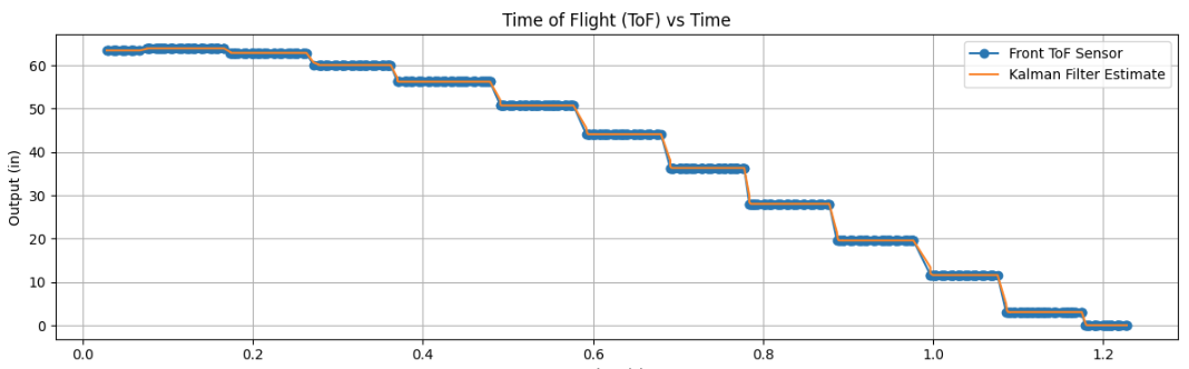
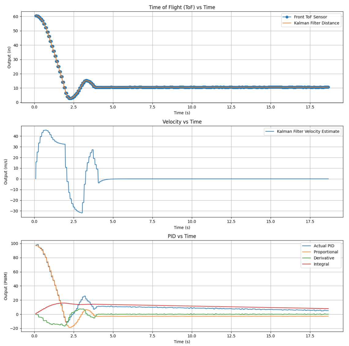
    return mu, sigma

The figure below is where I will place the Kalman Filter comparison plot between the raw sensor signal and the estimated state.

6. Kalman Filter on the Robot

After testing the Kalman Filter in Python, I implemented it on the Artemis using matrix math. This let the robot estimate distance and velocity during the control loop instead of waiting only on the next raw ToF update.

This was useful because the ToF sensor updates more slowly than the controller can run. With the Kalman Filter, I could use an estimated state that updated continuously and gave smoother behavior.

Matrix Operations on the Robot

#include <BasicLinearAlgebra.h>
using namespace BLA;

Matrix<2,1> state = {0,0};
Matrix<1> u;
Matrix<2,2> A = {1, 1,
                 0, 1};

Sigma_p = Ad * Sigma * ~Ad + Sigma_u;

7. Discussion

Overall, the Kalman Filter improved the robot’s state estimate by combining model prediction with measured sensor data. Compared to relying on only the raw ToF sensor, the Kalman Filter gave a cleaner estimate of both position and velocity.

One of the most important parts of this lab was tuning the covariance matrices. If the process noise was too small, the filter responded too slowly. If the measurement noise was too small, the filter trusted the sensor too much and became noisier.

This lab also showed why a model-based estimate can be more useful than simple extrapolation. The Kalman Filter gave a better estimate between sensor updates and set up the robot for faster control in the next lab.

These are my plots from the Kalman Filter implementation:

8. Video Demonstration

Kalman Filter Test Video

9. Acknowledgments

I used ChatGPT to help structure parts of my code, debug implementation issues, and assist with generating and interpreting plots in Python. It was mainly used as a tool to help understand concepts and speed up development, not to replace my understanding of the material.

I also worked with Pages Ethan Sarpong and Andrew Donofrio, who helped with executing different parts of the lab and troubleshooting hardware and implementation issues.

Lab 7: Kalman Filter