Lab 12: Inverted Pendulum

The goal of this lab was to use the robot's closed-loop control capabilities to perform an inverted pendulum style stunt. Instead of doing path planning and navigation, this lab focused on controls, estimation, and tuning so the robot could lift onto two wheels and try to maintain a wheelie position.

My approach was to recycle the orientation control structure from Lab 6, but instead of controlling yaw, I used the IMU's DMP quaternion output to estimate pitch. This allowed the robot to react to pitch error and drive forward or backward to move itself closer to the balancing angle.

To measure the robot's angle during the wheelie, I used the IMU's onboard Digital Motion Processor. The DMP outputs quaternion data, which can be converted into pitch. This was better than just integrating raw gyroscope data because the raw gyro can drift over time and make the angle estimate less reliable.

I used the quaternion values to calculate pitch, then calibrated the pitch measurement so the robot's measured range better matched the real physical angle of the robot.

double t0 = +2.0 * (qw * qx + qy * qz);
double t1 = +1.0 - 2.0 * (qx * qx + qy * qy);

Gyro_pitch = atan2(t0, t1) * 180.0 / PI;

IMU / Robot Setup

Pitch Reading Test

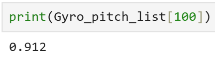
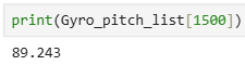
The next step was to calibrate the DMP pitch readings. When the robot was placed flat at what should have been 0 degrees, the DMP read 0.912 degrees. When the robot was placed against the wall at what should have been 90 degrees, the DMP read 89.243 degrees.

To correct this, I mapped the measured range from 0.912 → 89.243 to the desired range of 0 → 90. This made the pitch value more useful for the controller.

Gyro_pitch = (atan2(t0, t1) * 180.0 / PI - 0.912f) * 90.0f / (89.243f - 0.912f);

After this correction, I found that the robot did not balance perfectly at exactly 90 degrees because of the weight distribution from the electronic components. Through trial and error, I found that adding about 1 to 1.5 degrees helped the robot reach equilibrium more consistently.

Gyro_pitch = (atan2(t0, t1) * 180.0 / PI - 0.912f) * 90.0f / (89.243f - 0.912f) + 1.0f;

0 Degree Calibration

90 Degree Calibration

I created a new case named WHEELEE where I placed the inverted pendulum control logic. The controller calculated the error between the measured pitch angle and the target wheelie angle. Depending on the sign of the error, the robot would drive forward or backward to correct itself.

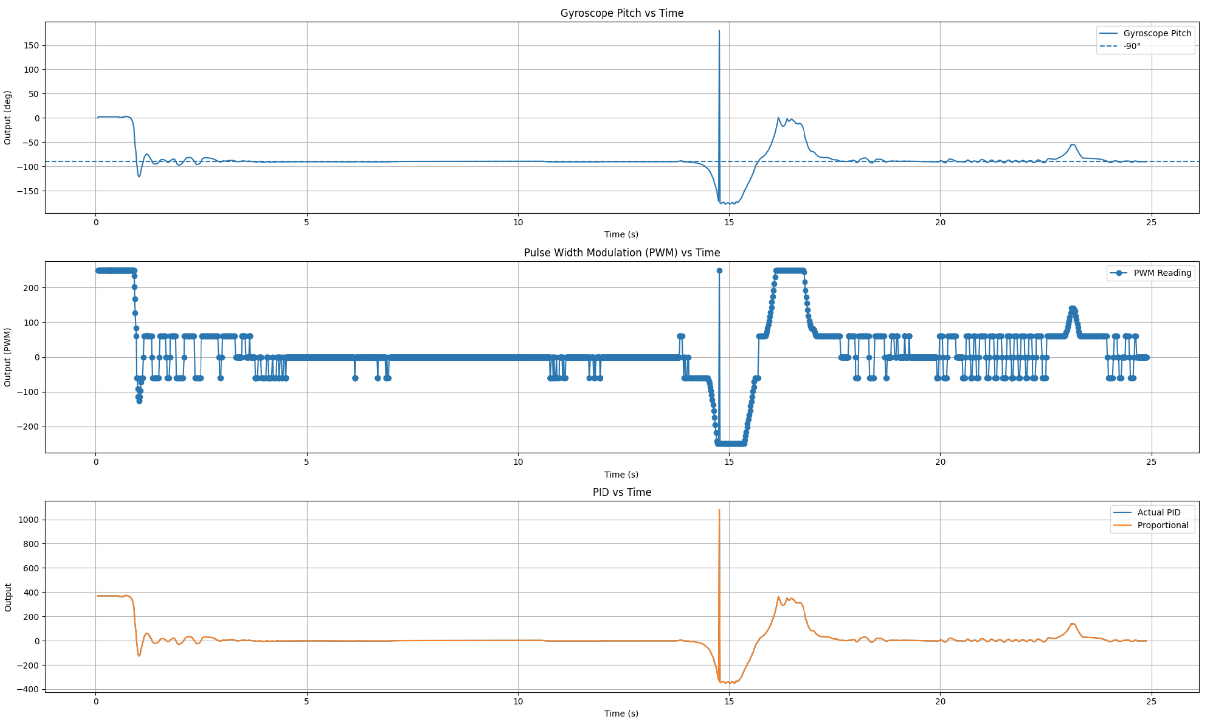
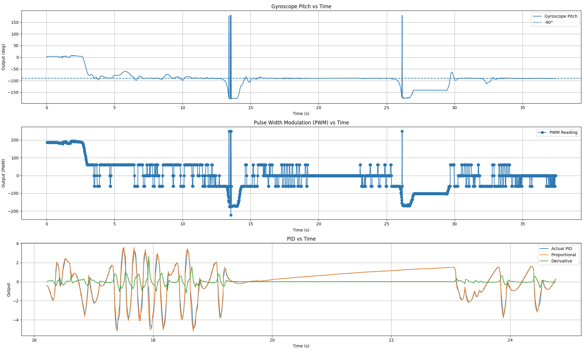
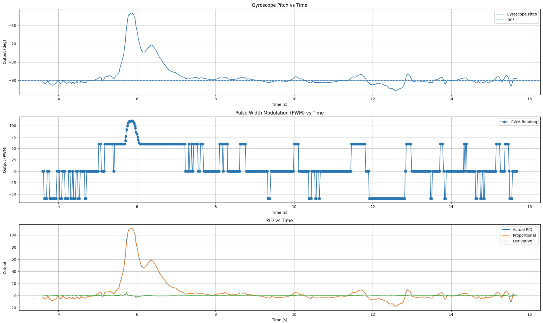
The values I logged included time, gyroscopic pitch, total PID output, proportional error, integral error, derivative error, and motor PWM output. This made it easier to compare different gain values and understand how the robot was responding.

error1P_ori = Gyro_pitch - targetOrientation1;

static unsigned long PID_time2_ori = millis();
unsigned long PID_time1_ori = millis();

PID_dt_ori = (PID_time1_ori - PID_time2_ori) / 1000.0;
error1I_ori += error1P_ori * PID_dt_ori;

if (PID_dt_ori > 0) {
  error1D_ori = (error1P_ori - error1Plast_ori) / PID_dt_ori;
}

error1Plast_ori = error1P_ori;

if (error1I_ori > 4000) error1I_ori = 4000;
if (error1I_ori < -4000) error1I_ori = -4000;

PID_time2_ori = PID_time1_ori;

float control_ori = (kp_ori * error1P_ori) +
                    (ki_ori * error1I_ori) +
                    (kd_ori * error1D_ori);

duty2 = abs(control_ori);

if (duty2 < duty1Min_drive) duty2 = duty1Min_drive;
if (duty2 > duty1Max_drive) duty2 = duty1Max_drive;

Since the robot only needed small angle corrections near the balancing point, I decided not to use integral control in my final tuning. Integral control was not as useful for this stunt because it could build up error and cause the robot to overshoot more, especially since the robot needed quick small corrections instead of slow steady-state correction.

float deadband_ori = 1.25;

if (fabs(error1P_ori) <= deadband_ori) {
  stop_motors();
}
else {
  if (error1P_ori > 0) {
    drive_forward(duty2);
  }
  else {
    drive_backward(duty2);
  }
}

Since I recycled parts of my Lab 6 orientation control code, the original minimum PWM value was too high for this task. At first, the minimum PWM was around 170, which made the robot react too aggressively and spaz out. After testing, I brought the minimum PWM down to the driving minimum from Lab 4, which was around 60.

I also tested different deadband values from about 0.5 degrees to 1.5 degrees. A smaller deadband made the controller more sensitive, but it also caused more oscillation near the target angle. I ended up using a deadband of 1.25 degrees, which gave the robot enough room to settle without constantly twitching.

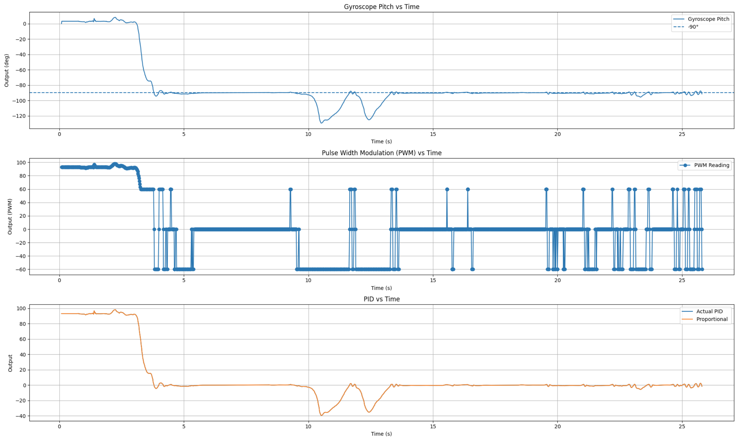
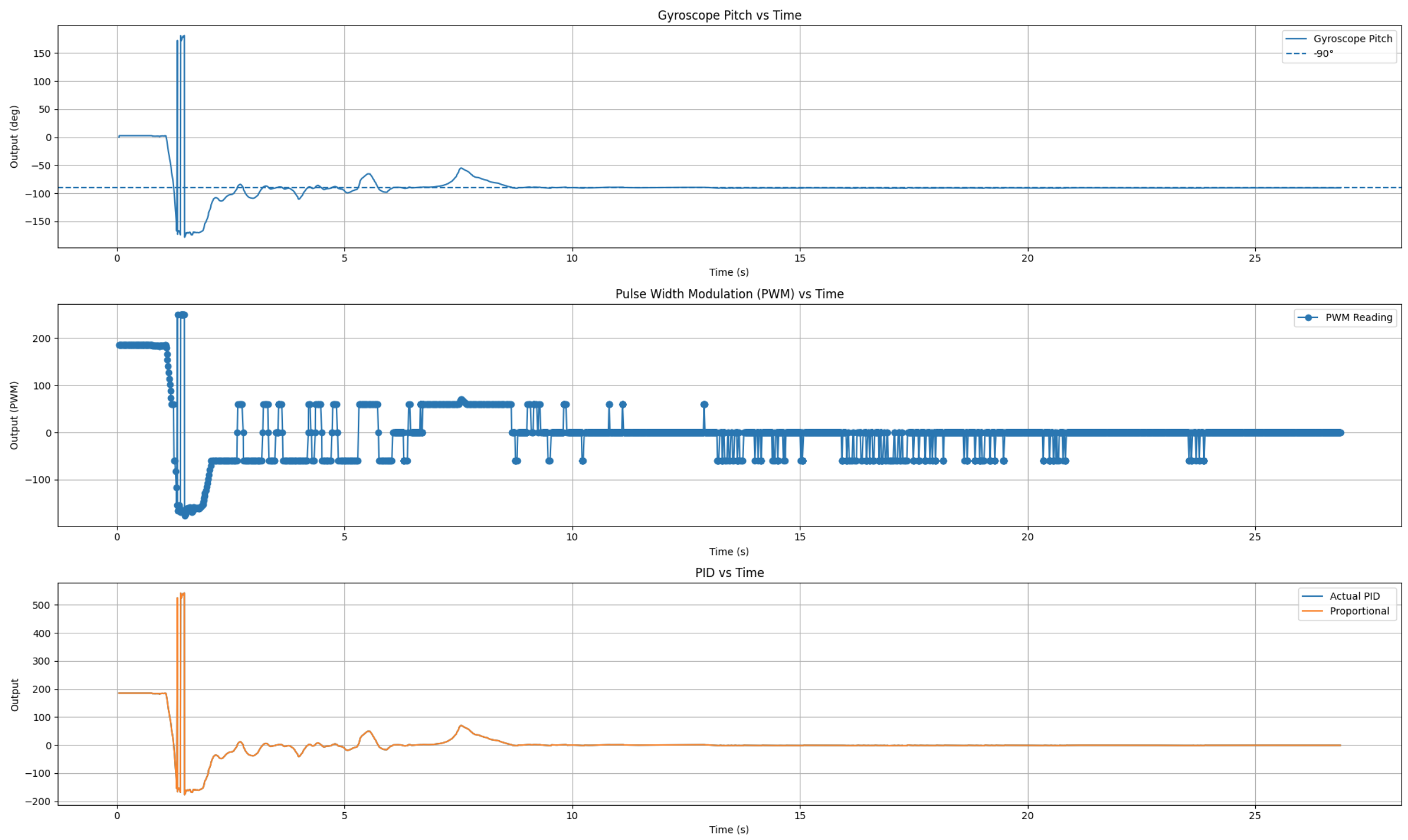
I started tuning with proportional control on carpet. I tested Kp = 1.0, Kp = 2.0, and Kp = 4.0. The Kp = 1.0 response was too weak and the robot did not always react strongly enough. The Kp = 4.0 response was stronger, but it caused more overshoot and oscillation. I ended up using Kp = 2.0 because it gave a better balance between response strength and stability.

Test 1: Kp = 1.0

Test 2: Kp = 2.0

Test 3: Kp = 4.0

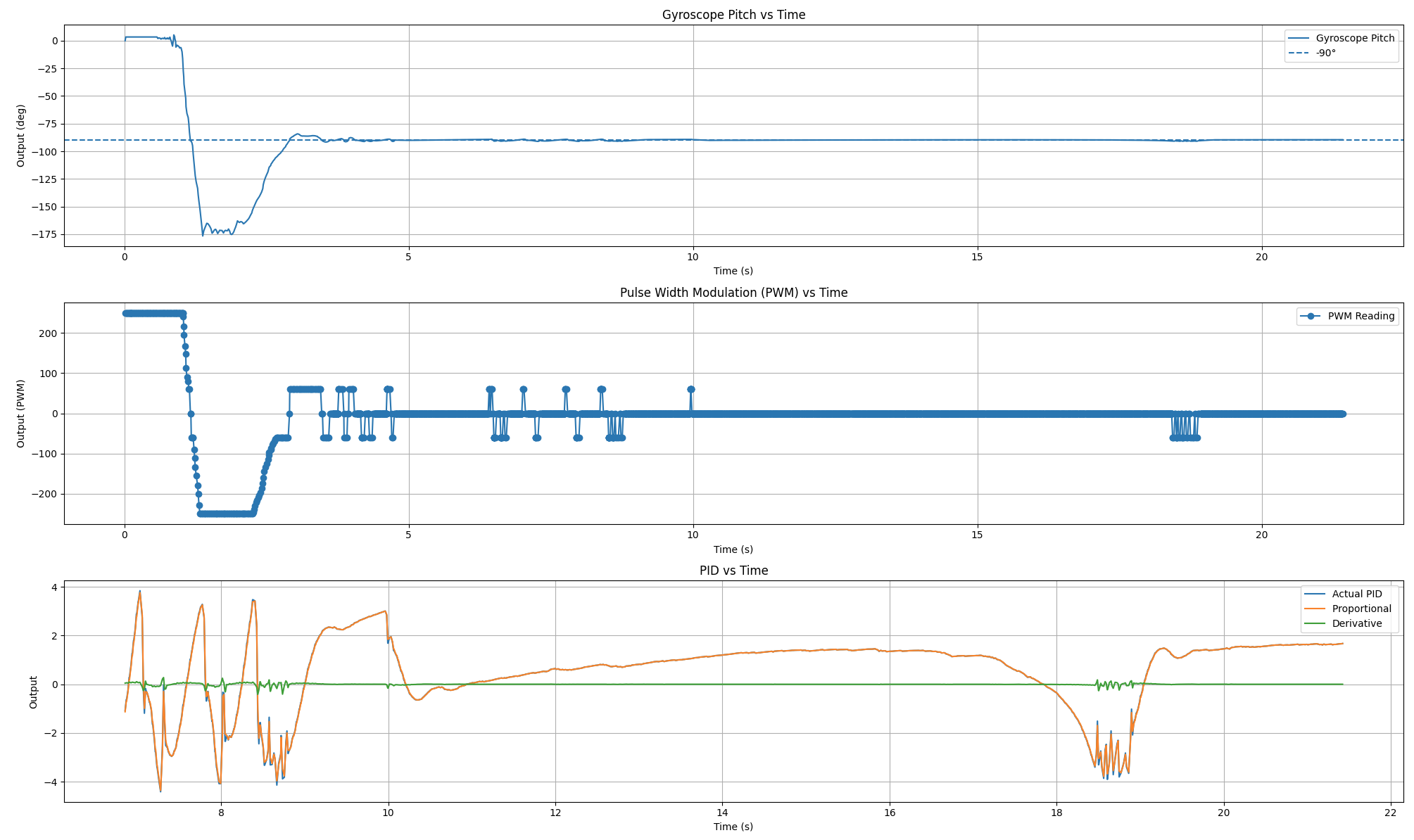
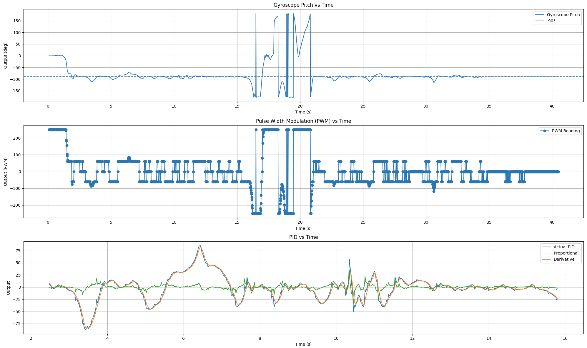
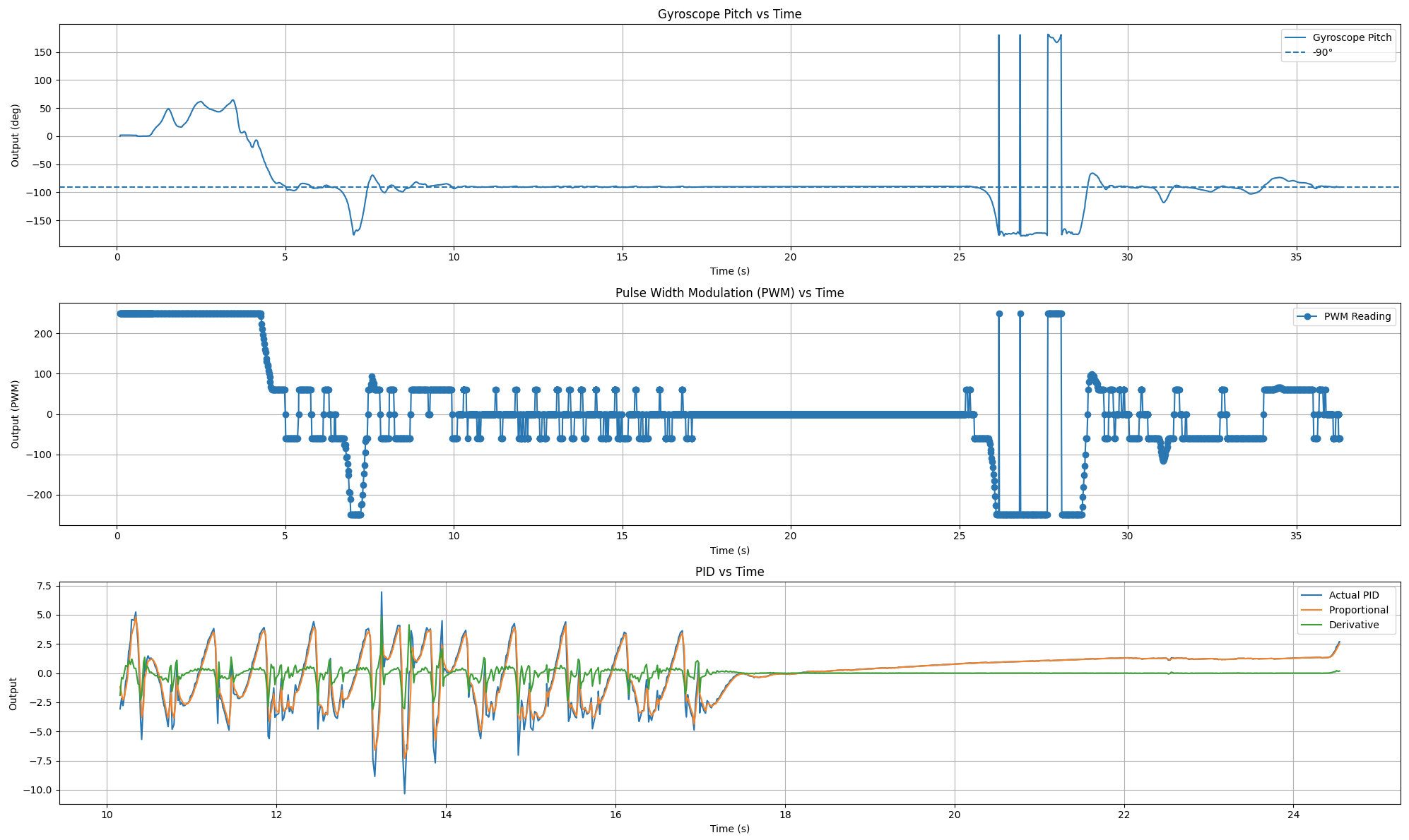
After choosing the proportional gain, I tested derivative control. The derivative term helped add a quicker response when the robot started falling away from the target angle. This was useful because when the robot reached larger errors, such as around 20 degrees away from the balancing point, it sometimes needed a sharper correction to return toward equilibrium.

I tested Kd = 0.001, Kd = 0.005, and Kd = 0.01. I found that Kd = 0.005 gave a solid response on carpet without making the robot too jumpy.

Test 1: Kd = 0.001

Test 2: Kd = 0.005

Test 3: Kd = 0.01

For my final setup, I used Kp = 2.0 and Kd = 0.005. I tested the robot on carpet first because the higher friction helped the wheels grip the ground and gave the robot more control while trying to stay near equilibrium. The carpet also helped the robot remain upright slightly longer because it reduced slipping.

I also tested the robot on a smoother table surface. The table had less friction, so the robot had a harder time maintaining balance. The wheels could move more easily, but the robot also slipped more and had less time to correct itself before falling out of the wheelie position.

Final Carpet Data

Final Table Data

Overall, the inverted pendulum task was much harder than normal orientation control because the robot had to correct itself very quickly while balancing near an unstable point. Small errors in pitch caused the robot to fall forward or backward, so the controller had to react fast without creating too much overshoot.

The DMP pitch estimate made the control signal cleaner than raw gyroscope integration, but the robot was still limited by loop speed, motor response, friction, and the robot's weight distribution. The final controller worked best on carpet because the surface gave the wheels more grip and made the response easier to control.

If I continued improving this lab, I would try filtering the pitch signal more carefully, testing derivative-on-measurement to reduce derivative kick, and tuning the controller separately for different surfaces. I would also test different battery and electronics placements to move the center of mass closer to a more stable balancing point.